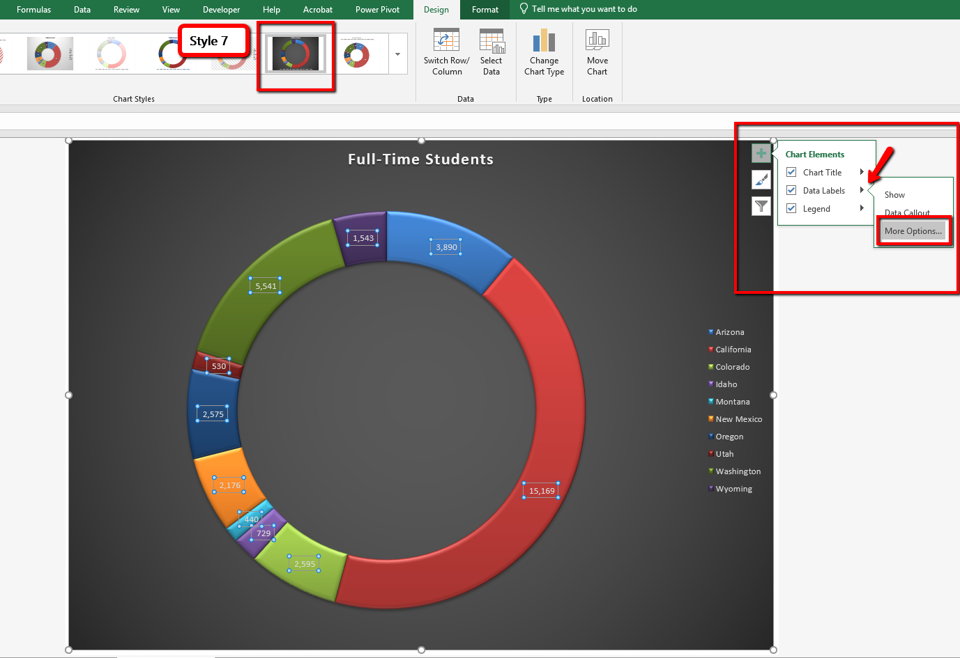
43 how to add data labels to a pie chart in excel on mac
How to set the chart of spreadsheet | WPS Office Academy Select the cells that contain the data you'd like to use so as to create a chart. Click Insert tab, then click Chart to select the type of chart that fits the content. (In this example, we choose a pie chart that matches with percentage description). 2. In the pop-up chart page, click the first icon Chart Elements in the right border to add ... How to Apply a Filter to a Chart in Microsoft Excel - How-To Geek Select the data for your chart, not the chart itself. Go to the Home tab, click the Sort & Filter drop-down arrow in the ribbon, and choose "Filter." Click the arrow at the top of the column for the chart data you want to filter. Use the Filter section of the pop-up box to filter by color, condition, or value.
Adding Text Boxes to Charts (Microsoft Excel) - tips Simply make sure it is displayed, then click the Text Box tool. The mouse pointer changes to crosshairs, and you can click and drag to outline the text box you want created. The second way to create a text box is to use the Formula bar. Make sure you select any part of your chart except a title or data label. Click in the Formula bar and start ...

How to add data labels to a pie chart in excel on mac
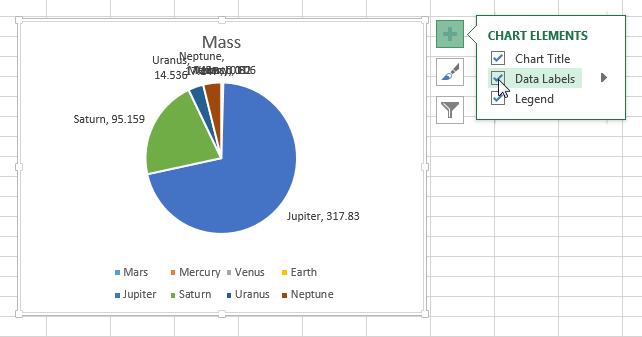
EOF How do you make a pie chart in Excel with percentages? To add data labels, select the chart and then click on the "+" button in the top right corner of the pie chart and check the Data Labels button. It can be observed that the pie chart contains the value in the labels but our aim is to show the data labels in terms of percentage. Status and trend work item, query-based charts - Azure DevOps Select the Chart for work items widget and then select Add. Select the widget's gear icon to open the Configuration dialog. Give the chart a title, select the flat list query on which the chart is based, and choose the chart type. Based on your chart type, specify values for the remaining fields.
How to add data labels to a pie chart in excel on mac. How to Make a Pie Chart in Microsoft Excel - groovyPost Select the data you want to use for the chart. You can do this easily by dragging your cursor through the cell range. Go to the Insert tab and click the Pie Chart drop-down arrow. In Excel on the... How to Use Excel Pivot Table Label Filters - Contextures Excel Tips To change the Pivot Table option, and allow multiple filters, follow these steps: Right-click a cell in the pivot table, and click PivotTable Options. In the PivotTable Options dialog box, click the Totals & Filters tab In the Filters section, add a check mark to 'Allow multiple filters per field.' How to Insert Pie Chart in WPS Spreadsheet Click the data label in the chart, and click the Format Chart Area button. In the LABEL tab, we select Percentage. Then we can also change the chart style. 1. Click the Change Color drop-down button, and select a desired color type for the chart. 2. There are also some built-in styles for choice. Here we apply Style 12 to the chart. 3. Module 4 Stuarts Bank Analyze and Chart Financial Data SAM Project 1B ... Customize the combo chart as follows to clarify its data: a. Apply the Monochromatic Palette 3 color scheme to the chart. b. Add a secondary axis for the Total series. [Mac Hint: Select the Total series and use the format pane to add the axis.] c. Add Vertical Axis Titles to the chart, using Expenses per Category as the Left
How to Make a Pie Chart in Microsoft Excel - How-To Geek While your data is selected, in Excel's ribbon at the top, click the "Insert" tab. In the "Insert" tab, from the "Charts" section, select the "Insert Pie or Doughnut Chart" option (it's shaped like a tiny pie chart). Various pie chart options will appear. How to work on spreadsheet document using the information given Guided Project 3-3 Windows Mac Don't use plagiarized sources. Get Your Custom Essay on How to work on spreadsheet document using the information given Just from $13/Page Order Essay Blue Lake Sports has locations in several major cities and tracks sales by department in each store. For this project, you create a pie chart […] Add bevel, emboss, and texture styles to a paginated report chart ... To add bevel or emboss styles to a pie or doughnut chart. On the View tab, select Properties to open the Properties pane. Select the pie or doughnut chart that you want to enhance. Select a data field in the chart, not the entire chart. In the Properties pane, expand the CustomAttributes node. For PieDrawingStyle, select a style from the drop ... How to Make a Pie Chart in Excel & Add Rich Data Labels to The Chart! Creating and formatting the Pie Chart. 1) Select the data. 2) Go to Insert> Charts> click on the drop-down arrow next to Pie Chart and under 2-D Pie, select the Pie Chart, shown below. 3) Chang the chart title to Breakdown of Errors Made During the Match, by clicking on it and typing the new title.
How To Show Two Sets of Data on One Graph in Excel Below are steps you can use to help add two sets of data to a graph in Excel: 1. Enter data in the Excel spreadsheet you want on the graph. To create a graph with data on it in Excel, the data has to be represented in the spreadsheet. For multiple variables that you want to see plotted on the same graph, entering the values into different ... How to Create and Customize a Pie Chart in Google Sheets - MUO Start by selecting the cells containing the information. Open the Insert menu and click Chart. Google Sheets will create a chart based on your data. Usually, the default chart isn't a pie chart but don't worry as we'll change that in a few clicks. Double-click the chart to bring up the Chart editor window. How to Edit Pie Chart in Excel (All Possible Modifications) 7. Change Data Labels Position. Just like the chart title, you can also change the position of data labels in a pie chart. Follow the steps below to do this. 👇. Steps: Firstly, click on the chart area. Following, click on the Chart Elements icon. Subsequently, click on the rightward arrow situated on the right side of the Data Labels option ... Pie Chart in Excel - Inserting, Formatting, Filters, Data Labels Click on the Instagram slice of the pie chart to select the instagram. Go to format tab. (optional step) In the Current Selection group, choose data series "hours". This will select all the slices of pie chart. Click on Format Selection Button. As a result, the Format Data Point pane opens.
Bar Graph No Labels - Free Table Bar Chart
Pie of Pie Chart in Excel - Inserting, Customizing - Excel Unlocked Inserting a Pie of Pie Chart. Let us say we have the sales of different items of a bakery. Below is the data:-. To insert a Pie of Pie chart:-. Select the data range A1:B7. Enter in the Insert Tab. Select the Pie button, in the charts group. Select Pie of Pie chart in the 2D chart section.
4.1 Choosing a Chart Type – Beginning Excel 2019
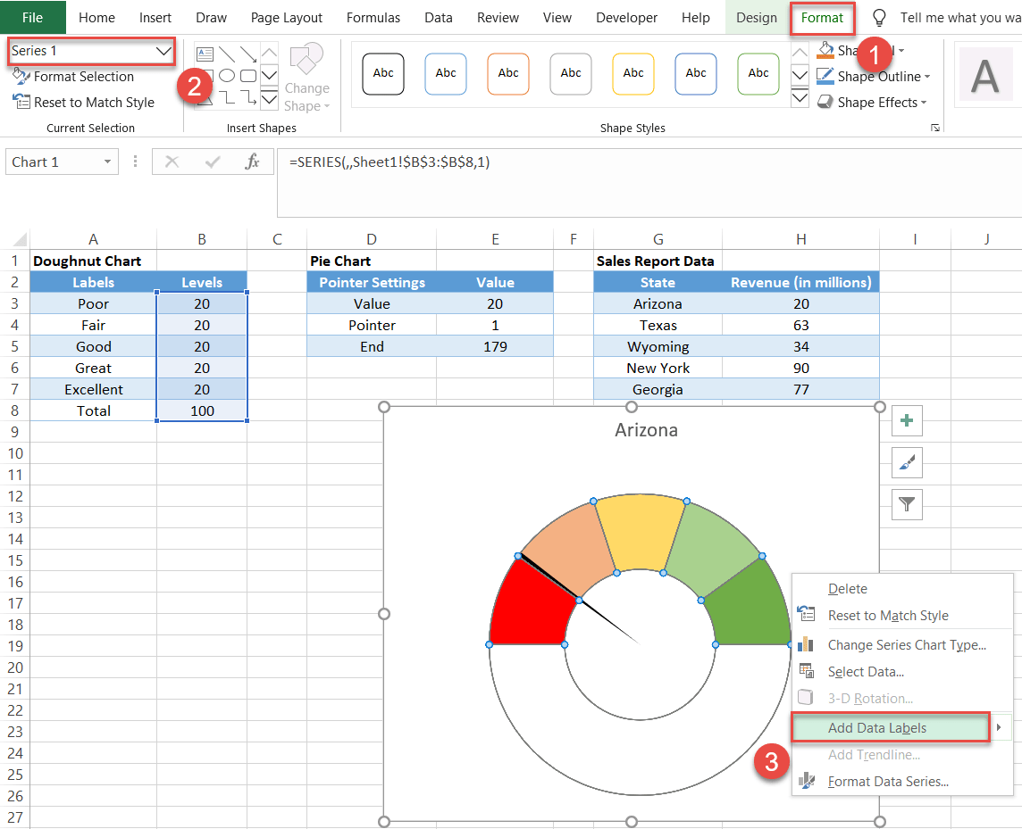
How To Make A Gauge Chart In Excel (Windows + Mac) Right click on the chart and click select data. Add a new legend series by pressing the plus icon. Then highlight the three values. Change chart type to a pie chart. Move the pie chart to the secondary axis by clicking on it and selecting secondary axis in the format data series panel.
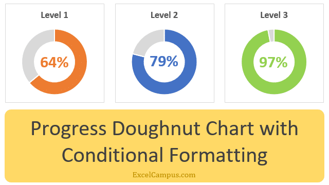
Charts & Dashboards Archives - Page 2 of 5 - Excel Campus
Status and trend work item, query-based charts - Azure DevOps Select the Chart for work items widget and then select Add. Select the widget's gear icon to open the Configuration dialog. Give the chart a title, select the flat list query on which the chart is based, and choose the chart type. Based on your chart type, specify values for the remaining fields.
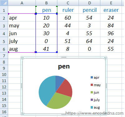
33 How To Label A Pie Chart In Excel - Labels 2021
How do you make a pie chart in Excel with percentages? To add data labels, select the chart and then click on the "+" button in the top right corner of the pie chart and check the Data Labels button. It can be observed that the pie chart contains the value in the labels but our aim is to show the data labels in terms of percentage.
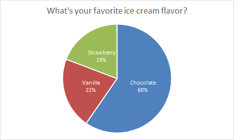
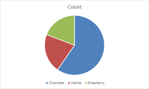
Pie Chart: Survey results favorite ice cream flavor | Exceljet
EOF
33 How To Label A Pie Chart In Excel - Labels 2021
Excel Gauge Chart Template - Free Download - How to Create
Pie Chart: Survey results favorite ice cream flavor | Exceljet
Post a Comment for "43 how to add data labels to a pie chart in excel on mac"