38 pie chart excel labels

Pie Chart in Excel - Inserting, Formatting, Filters, Data Labels Right click on the Data Labels on the chart. Click on Format Data Labels option. Consequently, this will open up the Format Data Labels pane on the right of the excel worksheet. Mark the Category Name, Percentage and Legend Key. Also mark the labels position at Outside End. This is how the chark looks. Formatting the Chart Background, Chart Styles How to Make a Pie Chart in Excel & Add Rich Data Labels to The Chart! Creating and formatting the Pie Chart 1) Select the data. 2) Go to Insert> Charts> click on the drop-down arrow next to Pie Chart and under 2-D Pie, select the Pie Chart, shown below. 3) Chang the chart title to Breakdown of Errors Made During the Match, by clicking on it and typing the new title.

Pie of Pie Chart in Excel - Inserting, Customizing - Excel Unlocked Inserting a Pie of Pie Chart. Let us say we have the sales of different items of a bakery. Below is the data:-. To insert a Pie of Pie chart:-. Select the data range A1:B7. Enter in the Insert Tab. Select the Pie button, in the charts group. Select Pie of Pie chart in the 2D chart section.

Pie chart excel labels

45 Free Pie Chart Templates (Word, Excel & PDF) ᐅ TemplateLab Click on Charts > Pie Charts to create a pie chart. Using Microsoft Word. Click on the "Insert" tab. Click the "Chart" button. On the left side, click "Pie" then choose the style that you want for your chart. On the new window that pops up, choose the style of your chart. How to Create a Pie Chart in Excel | Smartsheet Enter data into Excel with the desired numerical values at the end of the list. Create a Pie of Pie chart. Double-click the primary chart to open the Format Data Series window. Click Options and adjust the value for Second plot contains the last to match the number of categories you want in the "other" category. Inserting Data Label in the Color Legend of a pie chart Inserting Data Label in the Color Legend of a pie chart. Hi, I am trying to insert data labels (percentages) as part of the side colored legend, rather than on the pie chart itself, as displayed on the image below. Does Excel offer that option and if so, how can i go about it?

Pie chart excel labels. How to Make a PIE Chart in Excel (Easy Step-by-Step Guide) - Trump Excel Once you have the data in place, below are the steps to create a Pie chart in Excel: Select the entire dataset Click the Insert tab. In the Charts group, click on the 'Insert Pie or Doughnut Chart' icon. Click on the Pie icon (within 2-D Pie icons). The above steps would instantly add a Pie chart on your worksheet (as shown below). spreadsheeto.com › pie-chartHow To Make A Pie Chart In Excel. - Spreadsheeto How To Make A Pie Chart In Excel. In Just 2 Minutes! Written by co-founder Kasper Langmann, Microsoft Office Specialist. The pie chart is one of the most commonly used charts in Excel. Why? Because it’s so useful 🙂. Pie charts can show a lot of information in a small amount of space. They primarily show how different values add up to a whole. excel - How to not display labels in pie chart that are 0% - Stack Overflow Generate a new column with the following formula: =IF (B2=0,"",A2) Then right click on the labels and choose "Format Data Labels". Check "Value From Cells", choosing the column with the formula and percentage of the Label Options. Under Label Options -> Number -> Category, choose "Custom". Under Format Code, enter the following: › pie-chart-examplesPie Chart Examples | Types of Pie Charts in Excel with Examples It is similar to Pie of the pie chart, but the only difference is that instead of a sub pie chart, a sub bar chart will be created. With this, we have completed all the 2D charts, and now we will create a 3D Pie chart. 4. 3D PIE Chart. A 3D pie chart is similar to PIE, but it has depth in addition to length and breadth.

How to Create and Format a Pie Chart in Excel - Lifewire Select the plot area of the pie chart. Right-click the chart. Select Add Data Labels . Select Add Data Labels. In this example, the sales for each cookie is added to the slices of the pie chart. Change Colors When a chart is created in Excel, or whenever an existing chart is selected, two additional tabs are added to the ribbon. › Make-a-Pie-Chart-in-ExcelHow to Make a Pie Chart in Excel: 10 Steps (with Pictures) Add your data to the chart. You'll place prospective pie chart sections' labels in the A column and those sections' values in the B column. For the budget example above, you might write "Car Expenses" in A2 and then put "$1000" in B2. The pie chart template will automatically determine percentages for you. 5 Finish adding your data. Formatting data labels and printing pie charts on Excel for Mac 2019 ... Here's a work around I found for printing pie charts. Still can't find a solution for formatting the data labels. 1. When printing a pie chart from Excel for mac 2019, MS instructions are to select the chart only, on the worksheet > file > print. Excel is supposed to print the chart only (not the data ) and automatically fit it onto one page. › pie-chart-in-excelPie Chart in Excel | How to Create Pie Chart | Step-by-Step ... Excel Pie Chart ( Table of Contents ) Pie Chart in Excel; How to Make Pie Chart in Excel? Pie Chart in Excel. Pie Chart in Excel is used for showing the completion or main contribution of different segments out of 100%. It is like each value represents the portion of the Slice from the total complete Pie. For Example, we have 4 values A, B, C ...

Excel 2010 pie chart data labels in case of "Best Fit" Based on my tested in Excel 2010, the data labels in the "Inside" or "Outside" is based on the data source. If the gap between the data is big, the data labels and leader lines is "outside" the chart. And if the gap between the data is small, the data labels and leader lines is "inside" the chart. Regards, George Zhao. TechNet Community Support. Only Display Some Labels On Pie Chart - Excel Help Forum Only Display Some Labels On Pie Chart. I have a pie chart that contains over 50 categories (Yes, I know pie charts shouldn't be used for that many things) but I want to only display labels for maybe the top 5 values or any label with a value >10. This is because there are a few standout values but I want all the other values to remain in the ... How To Make A Pie Chart In Excel - lio.io How to Make a Pie Chart in Excel 1. Create columns and/or rows of data. Label each column of data as excel will use those labels as titles for your pie chart. Highlight the data you want to display in pie chart form. 2. Click "Insert" and then click on the "Pie". 3. Opt from the 2-dimensional and 3-dimensional pie. 4. And done. How to Create Bar of Pie Chart in Excel? Step-by-Step From the Insert tab, select the drop down arrow next to 'Insert Pie or Doughnut Chart'. You should find this in the 'Charts' group. From the dropdown menu that appears, select the Bar of Pie option (under the 2-D Pie category). This will display a Bar of Pie chart that represents your selected data.

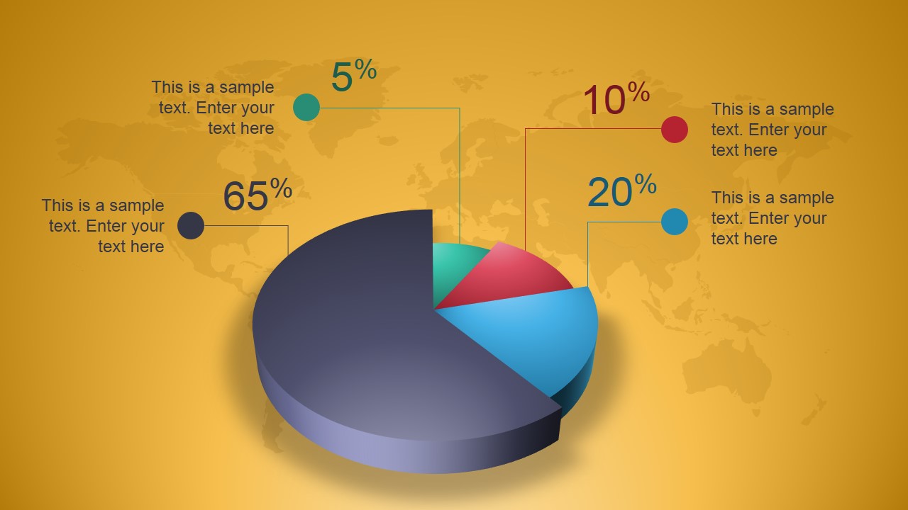
Creative 3D Perspective Pie Chart for PowerPoint - SlideModel

Office: Display Data Labels in a Pie Chart - Tech-Recipes: A Cookbook ... 3. In the Chart window, choose the Pie chart option from the list on the left. Next, choose the type of pie chart you want on the right side. 4. Once the chart is inserted into the document, you will notice that there are no data labels. To fix this problem, select the chart, click the plus button near the chart's bounding box on the right ...

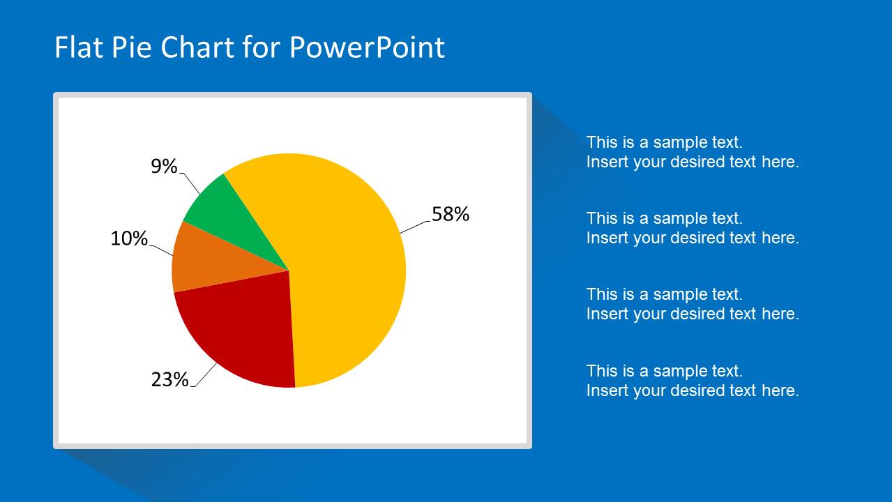
Flat Pie Chart Template for PowerPoint - SlideModel

› how-to-show-percentage-inHow to Show Percentage in Pie Chart in Excel? - GeeksforGeeks Jun 29, 2021 · Select a 2-D pie chart from the drop-down. A pie chart will be built. Select -> Insert -> Doughnut or Pie Chart -> 2-D Pie. Initially, the pie chart will not have any data labels in it. To add data labels, select the chart and then click on the “+” button in the top right corner of the pie chart and check the Data Labels button.

Pie Chart

Excel custom pie chart labels - Microsoft Community Excel custom pie chart labels I have a data set like this (basically form output): I want to use a pivot table to make a pie chart out of this. I want each of the pieces of the pie to contain the number of entries and between parentheses the percentage. So in the "Yes" piece, there should be '3 (33%)'.

Microsoft Excel Tutorials: How to Create a Pie Chart

How to☝️Create a Pie of Pie Chart in Excel - SpreadsheetDaddy Let's take a look at how to add data points to your chart. Right-click on the chart. Select the Add Data Labels option. If you want the labels to be more visually appealing, you can change their color as well. Select the labels. Go to the Home menu. Navigate to the Font section and click on the Font Color option.

Excel rotate radar chart - Stack Overflow

Chart Legend / Data Labels In Pie Chart | MrExcel Message Board Jun 6, 2009. #3. Add the data labels. Then, right click on any data label to select all the data labels for that series and select Format Data Labels... From the Label Options tab, in the Label Contains section, select the 'Series Name' checkbox. The above applies to Excel 2007. Excel 2003 supports the same capability though the dialog box ...

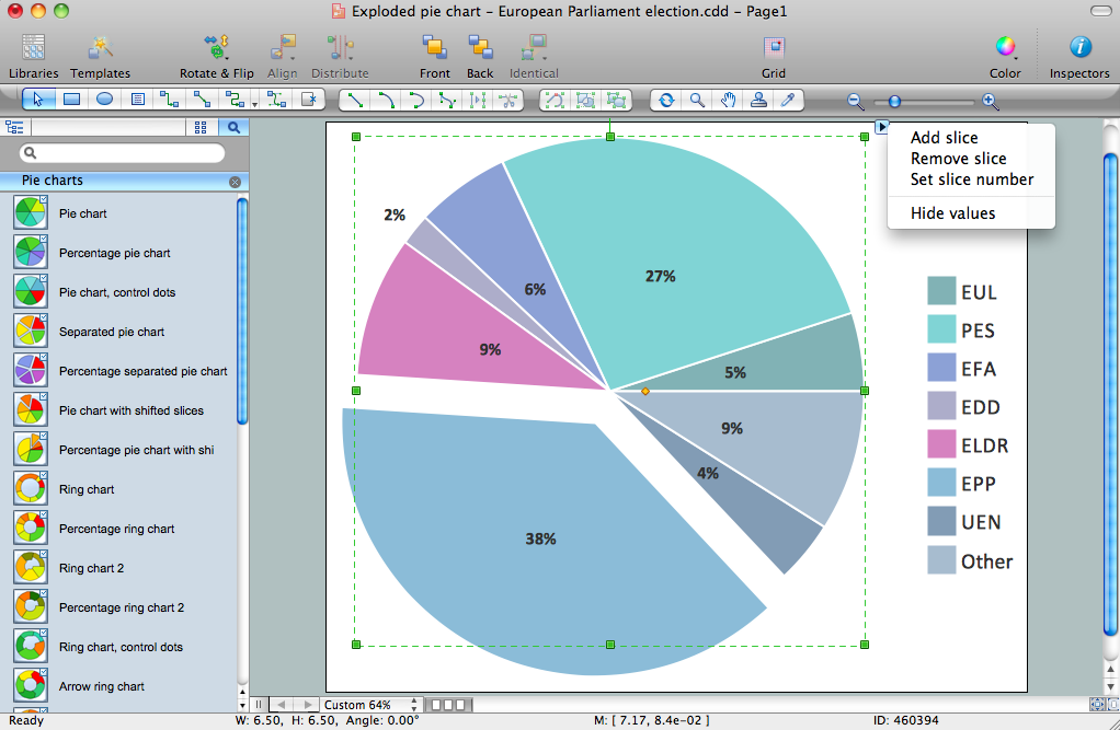
Pie Chart Software | Pie Charts, Donut Charts

Add or remove data labels in a chart - support.microsoft.com Click the data series or chart. To label one data point, after clicking the series, click that data point. In the upper right corner, next to the chart, click Add Chart Element > Data Labels. To change the location, click the arrow, and choose an option. If you want to show your data label inside a text bubble shape, click Data Callout.

How to Add Data Labels to an Excel 2010 Chart - dummies

› examples › pie-chartCreate a Pie Chart in Excel (In Easy Steps) - Excel Easy 6. Create the pie chart (repeat steps 2-3). 7. Click the legend at the bottom and press Delete. 8. Select the pie chart. 9. Click the + button on the right side of the chart and click the check box next to Data Labels. 10. Click the paintbrush icon on the right side of the chart and change the color scheme of the pie chart. Result: 11.

Share :